Model reduction¶

Linear reduced-order models¶

We provide a class to find reduced-order models (continuous and discrete time) by projecting linear dynamics onto modes (Petrov-Galerkin projection). The governing equation of the full system is assumed to be either continuous time:

$\partial x(t)/ \partial t &= A x(t) + B u(t) \\ y(t) &= C x(t)$

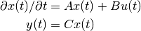
or discrete time:

$x(k+1) &= A x(k) + B u(k) \\ y(k) &= C x(k)$

where $k$ is the time step. Here $x$ is the state vector. $A$ , $B$ , and $C$ are, in general, linear operators (often arrays). In cases where there are no inputs and outputs, $B$ and $C$ are zero. $A$ acts on $x$ and returns a vector that lives in the same vector space as $x$ . $B$ acts on elements of the input space, $\mathbb{R}^p$ , where $p$ is the number of inputs and returns elements of the vector space in which $x$ lives. $C$ acts on $x$ and returns elements of the output space, $\mathbb{R}^q$ , where $q$ is the number of outputs.

These dynamical equations can be projected onto a set of modes. First, approximate the state vector as a linear combination of $r$ modes, stacked as columns of array $\Phi$ , and time-varying coefficients $q(k)$ :

$x(k) \approx \Phi q(k) .$

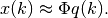
Then substitute into the governing equations and take the inner product with a set of adjoint modes, columns of array $\Psi$ . The result is a reduced system for $q$ , which has as many elements as $\Phi$ has columns, $r$ . The adjoint, $(\,\,)^+$ , is defined with respect to inner product weight $W$ .

$q(k+1) &= A_r q(k) + B_r u(k) \\ y(k) &= C_r q(k) \\ \text{where} \\ A_r &= (\Psi^+ \Phi)^{-1} \Psi^+ A \Phi \\ B_r &= (\Psi^+ \Phi)^{-1} \Psi^+ B \\ C_r &= C \Phi$

An analagous result exists for continuous time.

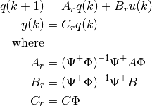
If the modes are not stacked into arrays, then the following equations are used, where $[\,\,]_{i,j}$ denotes row $i$ and column $j$ .

$[\Psi^+ \Phi]_{i,j} &= \langle\psi_i,\, \phi_j \rangle_W \\ [\Psi^+ A \Phi]_{i,j} &= \langle\psi_i,\, A \phi_j\rangle_W \\ [\Psi^+ B] &= \langle \psi_i,\, B e_j\rangle_W \\ [C \Phi]_{:,j} &= C \phi_j$

$e_j$ is the jth standard basis (intuitively $B e_j$ is $[B]_{:,j}$ if $B$ is an array.).

The $A$ , $B$ , and $C$ operators may or may not be available within Python. For example, you may do simulations using code written in another language. For this reason, modred requires only the action of the operators on the vectors, i.e., the products $A \phi_j$ , $Be_j$ , and $C \phi_j$ , and not the operators $A$ , $B$ , and $C$ themselves.

Example 1: Smaller data and arrays¶

Here’s an example that uses arrays.

import os

import numpy as np

import modred as mr


# Create directory for output files
out_dir = 'rom_ex1_out'
if not os.path.isdir(out_dir):
    os.makedirs(out_dir)

# Create random LTI system
nx = 100
num_inputs = 2
num_outputs = 3
num_basis_vecs = 10
A = np.random.random((nx, nx))
B = np.random.random((nx, num_inputs))
C = np.random.random((num_outputs, nx))

# Create random modes
basis_vecs = np.random.random((nx, num_basis_vecs))

# Perform Galerkin projection and save data
LTI_proj = mr.LTIGalerkinProjectionArrays(basis_vecs)
A_reduced, B_reduced, C_reduced = LTI_proj.compute_model(
    A.dot(basis_vecs), B, C.dot(basis_vecs))
LTI_proj.put_model(
    '%s/A_reduced.txt' % out_dir, '%s/B_reduced.txt' % out_dir,
    '%s/C_reduced.txt' % out_dir)

The array basis_vecs contains the vectors that define the basis onto which the dynamics are projected.

A few variations of this are illustrative. First, if no inputs or outputs exist, then there is only $A_r$ and no $B_r$ or $C_r$ . The last two lines would then be replaced with:

A_reduced = LTI_proj.reduce_A(A.dot(basis_vec_array))
LTI_proj.put_A_reduced('A_reduced.txt')

Another variant is if the basis vecs are known to be orthonormal, as is always the case with POD modes. Then, the $\Psi^* W \Phi$ array and its inverse are identity, and computing it is wasteful. Specifying the constructor keyword argument is_basis_orthonormal=True tells modred this array is identity and to not compute it.

Example 2: Larger data and vector handles¶

Here’s an example similar to what might arise when doing large simulations in another language or program.

import os

import numpy as np

from modred import parallel
import modred as mr


# Create directory for output files
out_dir = 'rom_ex2_out'
if not os.path.isdir(out_dir):
    os.makedirs(out_dir)

# Create handles for modes
num_modes = 10
basis_vecs = [
    mr.VecHandlePickle('%s/dir_mode_%02d.pkl' % (out_dir, i))
    for i in mr.range(num_modes)]
adjoint_basis_vecs = [
    mr.VecHandlePickle('%s/adj_mode_%02d.pkl' % (out_dir, i))
    for i in mr.range(num_modes)]

# Define system dimensions and create handles for action on modes
num_inputs = 2
num_outputs = 4
A_on_basis_vecs = [
    mr.VecHandlePickle('%s/A_on_dir_mode_%02d.pkl' % (out_dir, i))
    for i in mr.range(num_modes)]
B_on_bases = [
    mr.VecHandlePickle('%s/B_on_basis_%02d.pkl' % (out_dir, i))
    for i in mr.range(num_inputs)]
C_on_basis_vecs = [
    np.sin(np.linspace(0, 0.1 * i, num_outputs)) for i in mr.range(num_modes)]

# Create random modes and action on modes. Typically this data already exists
# and this section is unnecesary.
nx = 100
ny = 200
if parallel.is_rank_zero():
    for handle in (
        basis_vecs + adjoint_basis_vecs + A_on_basis_vecs + B_on_bases):
        handle.put(np.random.random((nx, ny)))
parallel.barrier()

# Perform Galerkin projection and save data to disk
inner_product = np.vdot
LTI_proj = mr.LTIGalerkinProjectionHandles(
    inner_product, basis_vecs, adjoint_basis_vec_handles=adjoint_basis_vecs)
A_reduced, B_reduced, C_reduced = LTI_proj.compute_model(
    A_on_basis_vecs, B_on_bases, C_on_basis_vecs)
LTI_proj.put_model(
    '%s/A_reduced.txt' % out_dir, '%s/B_reduced.txt' % out_dir,
    '%s/C_reduced.txt' % out_dir)

This example works in parallel with no modifications.

If you do not have the time-derivatives of the direct modes but want a continuous time model, see ltigalerkinproj.compute_derivs_arrays() and ltigalerkinproj.compute_derivs_handles().

Eigensystem Realization Algorithm (ERA)¶

See the documentation and examples provided in era.compute_ERA_model() and era.ERA.